
| 일 | 월 | 화 | 수 | 목 | 금 | 토 |
|---|---|---|---|---|---|---|
| 1 | 2 | 3 | 4 | 5 | 6 | |
| 7 | 8 | 9 | 10 | 11 | 12 | 13 |
| 14 | 15 | 16 | 17 | 18 | 19 | 20 |
| 21 | 22 | 23 | 24 | 25 | 26 | 27 |
| 28 | 29 | 30 |
- 실행계획 원리
- SQLServer
- fast in ssms
- Dataannotation
- .net
- identityserver
- execution plan
- identityserver3
- async await
- TPL
- async
- await
- SSMS
- slow in the application
- C#
- 영어공부
- 저장프로시저
- 쿼리 최적화
- ThreadPool
- task
- english
- IdentityServer4
- 느린 저장프로시저
- query
- oauth2
- esl
- stored procedure
- MSSQL
- SQL Server Optimizer
- validation
- Today
- Total
Genius DM
Slow in the Application, Fast in SSMS? Part 1 본문
어플리케이션에서는 느리고, SSMS 에서는 빠르다? Part 1
들어가기 전에
예제로 들어가기에 앞서 Northwind 샘플 데이터베이스를 사용했음을 알린다. 해당 데이터베이스는 SQL 2000 에 포함되어있다. 이후 버전은 Microsoft's web site. 에서 다운로드 할 수 있다. 포스트 내용의 핵심적인 것은 모든 버전의 SQL Server 에 적용되긴 하지만, 어쨌든 SQL 2005 혹은 그 이후 버전을 중점적으로 작성되었음을 알린다. 이 포스트에서는 캐싱 계획을 조사하는 몇 가지 쿼리를 다룬다. SQL 2000 이전 버전은 캐싱 계획 측면에서 매우 성능이 낮은 편이다. 포스트에서 제시하는 쿼리를 수행하기 위해서는 서버 상태를 조회할 수 있는 서버 레벨의 권한이 있어야 한다는 것을 기억하자.
이 포스트는 초보자 수준의 내용은 아니며, 어느정도 SQL 프로그래밍에 대한 실무 경력을 지니고 있는 사람은 읽을 수 있다. 성능 튜닝에 대한 경험이 반드시 필요한 것은 아니지만, 쿼리 계획에 대해 조금이라도 봤거나 인덱스에 대한 기본 지식이 있다면 이 포스트가 분명히 도움이 될 것이다. 여기서 다루는 내용은 기초 수준을 벗어나기 때문에, 기초 내용을 심도있게 다루지는 않을 것이다. 성능 튜닝에 대한 모든 것을 가르쳐주지도 않겠지만, 입문으로는 적합할 것이다.
주의: 포스트 곳곳에 Books Online 의 온라인 버전에 대한 링크를 삽입해두었다. 해당 URL 은 당신이 사용하는 SQL Server 버전과는 다른 버전의 내용을 보여줄지 모르지 주의하자. 토픽 페이지에서 다른 버전으로 이동할 수 있는 링크가 있으니 자신이 사용 중인 버전에 맞는 페이지로 이동하자 ( 적어도 MSDN 의 Books Online 이 내가 이 포스트를 작성한 시점에 그렇게 링크 배치를 했을지도 )
SQL Server 가 어떻게 저장 프로시저를 컴파일 하는가
이 챕터에서 어떻게 SQL Server 가 저장 프로시저를 컴파일하는지, 그리고 어떻게 캐싱 계획을 사용하는지 살펴볼 것이다. 만약 어플리케이션에서 SP 를 사용하지 않고 SQL 구문을 직접적으로 사용하더라도 이 챕터에서 이야기 하는 것 대부분이 도움이 될 것이다. 그러나 다이나믹 SQL 에서는 더 복잡한 문제가 있고, 저장 프로시저에 대한 것들도 충분히 어려워서 다이나믹 SQL 에 대한 내용은 별도의 챕터로 분리해 두었다.
저장 프로시저는 무엇인가?
질문이 좀 황당할 수 있다. 하지만 내가 볼 때 이 질문은 "어떤 것들이 쿼리 실행 계획을 포함하게 될까?" 와 동일하다. SQL 서버는 다음과 같은 타입에 쿼리 실행 계획을 포함시킨다.
- Scalar user-defined functions.
- Multi-step table-valued functions.
- Triggers.
좀 더 일반적이고 논리적인 용어로 모듈에 대해 얘기해야 하는데, 저장 프로시저가 가장 널리 사용되는 모듈 타입이라 간략하게 저장 프로시저에 대해서만 얘기하도록 하겠다. 위에서 제시한 3가지 객체 타입을 제외하면 SQL Server 에서 쿼리 실행 계획을 수립하는 경우는 없다. 특히 SQL Server 에서는 뷰와 인라인 테이블 함수에 대해 실행 계획을 작성하지 않는다.
SELECT abc, def FROM myview
SELECT a, b, c FROM mytablefunc(9)
위 쿼리는 테이블에 직접적으로 접근하는 AD-HOC 쿼리와 동일하다. SQL Server 는 쿼리를 컴파일 할 때 뷰 및 함수를 쿼리 내부로 확장하고 옵티마이저는 확장된 쿼리 문을 통해 동작한다. 저장 프로시저를 무엇이 만들어내는 것인지 이해하기 위해 한 가지 더 예제가 필요하다. 두 가지 프로시저가 있다고 가정해보자, 외부 프로시저가 내부 프로시저를 호출하는 예제이다.
CREATE PROCECURE Outer_sp AS
...
EXEC Inner_sp
...
대부분의 사람들이 Inner_sp 가 Outer_sp 와 독립적인 것이라고 생각할텐데, 실제로 그렇다. Other_sp 의 실행 계획은 Inner_sp 의 실행 계획을 포함하지 않고, 그저 호출 할 뿐이다. 하지만 비슷한 상황인데도 SQL 포럼 유저들이 동적 쿼리에 대해 매우 다르게 생각하는 경우가 있다.
CREATE PROCEDURE Some_sp AS
DECLARE @sql    nvarchar(MAX),
        @params nvarchar(MAX)
SELECT @sql = 'SELECT ...'
...
EXEC sp_executesql @sql, @params, @par1, ...
이게 내부 SP 와 동일하다고 이해하는 것이 중요하다. 생성된 SQL 문자열은 Some_sp 의 일부가 아니며, Some_sp 를 위한 쿼리 계획에서도 해당 문자열에 대한 계획은 찾아볼 수 없다. 다만 동적 쿼리 별도로 쿼리 실행 계획과 캐싱 진입점을 지닐 뿐이다. 이는 sp_executesql 을 통하거나 exec() 을 통해 실행되는 모든 동적 쿼리에 해당한다.
SQL Server 는 어떻게 실행 계획을 세우는가?
CREATE PROCEDURE ( 또는 CREATE FUNCTION 또는 CREATE TRIGGER ) 로 저장 프로시저를 만들면 SQL Server 는 코드가 문법적으로 올바른지 검사하고 존재하지 않는 컬럼을 참조했는지 여부를 검사한다. ( 만약 존재하지 않는 테이블을 참조했다면, Deferred Named Resolution 으로 불리는 기능으로 인해 에러는 발생하지 않는다. ) 하지만 생성 시점에서 쿼리 실행 계획을 세우진 않고, 데이터베이스에 해당 SQL 문을 저장할 뿐이다.
파라메터와 변수
Northwind 데이터베이스의 Orders 테이블과 아래 3개 프로시저를 보자.
CREATE PROCEDURE List_orders_1 AS
   SELECT * FROM Orders WHERE OrderDate > '20000101'
go
CREATE PROCEDURE List_orders_2 @fromdate datetime AS
   SELECT * FROM Orders WHERE OrderDate > @fromdate
go
CREATE PROCEDURE List_orders_3 @fromdate datetime AS
   DECLARE @fromdate_copy datetime
   SELECT @fromdate_copy = @fromdate
   SELECT * FROM Orders WHERE OrderDate > @fromdate_copy
goNote: SELECT 문에 별표 * 를 사용하는 것은 권장하지 않는다. 단지 예제를 심플하게 작성하기 위해서 사용했을 뿐이다.
그리고 아래 처럼 프로시저들을 실행해본다.
EXEC List_orders_1
EXEC List_orders_2 '20000101'
EXEC List_orders_3 '20000101'
프로시저를 실행하기 전에 쿼리 메뉴에 있는 실제 실행 계획 포함 을 활성화하고 실행한다. ( 툴바 버튼도 존재하고, Ctrl-M 이 단축키이다 ) 프로시저 실행 계획을 살펴보면, 위 첫 번째와 두 번째 프로시저의 실행계획이 동일하다는 것을 알 수 있다.
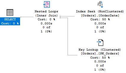
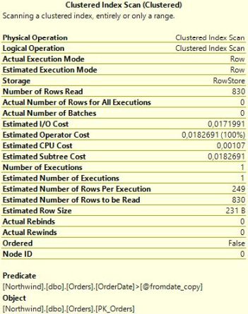
SQL Server 가 OrderDate 에 대한 인덱스를 탐색하고 Key lookup 을 사용해 다른 데이터를 가져왔음을 알 수 있다. 세 번째 프로시저의 실행계획은 좀 다르다.
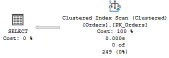
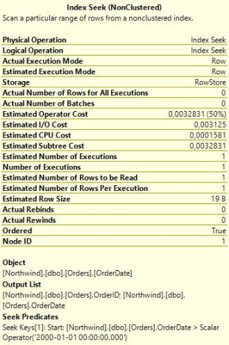
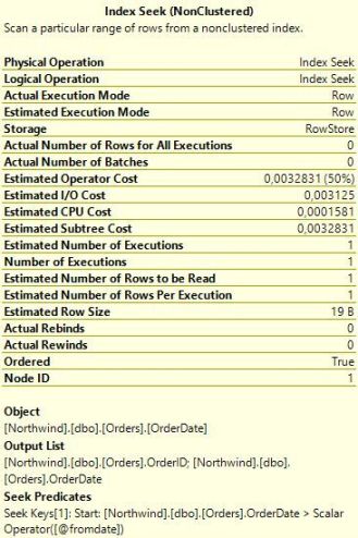
이 경우 SQL Server 가 테이블 스캔을 수행했다. ( 클러스터 인덱스에서는 Leaf page 가 데이터를 갖고 있음을 기억하자. 그렇기 때문에 클러스터 인덱스 스캔과 테이블 스캔을 근본적으로 동일하다. ) 왜 세 번째 실행 계획은 다른 것일까? 옵티마이저가 이러한 결정을 내린 이유를 이해하기 위해서 옵티마이저가 산출해낸 예상 내역을 보는 것이 좋다. Seek 연산자와 Scan 연산자에 마우스를 올리면 아래와 같은 팝업 창을 볼 수 있을 것이다.
 |  | |
| List_orders_1 | List_orders_2 | |
 | ||
| List_orders_3 | ||
Note: 정확한 내역은 어떤 SSMS 버전을 사용하느냐에 따라 다르다. 위 샘플들은 SQL Server 2008, 그리고 SSMS 2008 버전에서 구동한 화면이다. 최신 SSMS 버전을 사용한다면 항목들의 순서가 다소 다를 수 있고 더 많은 항목이 포함되어 있을 수도 있다. 추가 항목들은 샘플과는 전혀 관련이 없어서, 굳이 최신 버전의 예상 내역 화면을 사용하지 않고 2008년 버전의 스크린샷을 그대로 사용하고 있음을 알린다.
재미있는 항목은 바로 예상 행 수 이다. 1,2 번째 프로시저에서는 SQL Server 가 한 개의 행을 반환할 것이라고 계산했지만, 3번째 프로시저에서는 249개 행을 리턴할 것이라 계산했다. 이런 예상 수치 차이가 실행 계획에 있어 선택의 차이점을 설명해준다. Index seek + Key lookup 은 테이블에서 적은 양의 행을 반환하는 데 유용한 전략이다. 그러나 Seek 기준에 많은 수의 행이 매치되는 경우 비용이 증가하고 중복도가 높아지면서 SQL Server 는 동일한 데이터 페이지를 한 번 이상 접근하게 될 것이다. 모든 행이 리턴되는 케이스의 경우에는 Seek + Lookup 보다 테이블 스켄이 훨씬 효율적이다. 테이블 스캔에선 SQL Server 가 데이터 페이지를 정확히 한 번씩만 읽으면 된다. 반면에 Seek + Lookup 은 모든 페이지를 한 행 마다 한번 씩 읽어봐야 한다. Northwind 의 Orders 테이블은 830개의 행을 지니고 있고, SQL Server 가 249 행을 리턴할 것으로 계산한 경우, SQL Server 의 옵티마이저는 테이블 스캔이 가장 최적의 선택이라고 판단하게 되는 것이다.
이러한 예상수치는 어떻게 만들어지는가?
이제 옵티마이저가 쿼리 실행 계획을 왜 다르게 작성하는지 알게 되었다. 바로 예상수치가 다르기 때문이다. 그럼 바로 다음과 같은 의문을 가질 수 있다. 왜 예상 수치가 다른가? 바로 이것이 이 포스터의 핵심 주제이다. 첫 번째 프로시저에서 날짜는 상수였다. 즉, SQL Server 는 정확히 해당 날짜인 경우만 고려하면 되는 상황이였다. 따라서 SQL Server 는 Orders 테이블을 위한 통계 수치를 수집하고 이를 통해 2000년 대에 일치하는 OrderDate 가 없다는 것을 알아냈다. ( Northwind 데이터베이스의 데이터는 1996~1998 년 까지이다 ) 그러나 통계 수치는 통계 수치일 뿐, SQL Server 는 쿼리가 아예 한 개의 행도 반환하지 않을지에 대해 정확히 알 수 없다. 그래서 SQL Server 가 한 개의 행을 반환할 것이라고 예측한 것이다.
2번째 프로시저의 경우 변수를 사용하지 않고 파라메터를 사용했다. 최적화를 수행할 때 SQL Server 는 프로시저가 2000-01-01 이라는 파라메터 값과 함께 호출되었다는 사실은 알고 있다. 하지만 SQL Server 는 절차에 대한 분석은 수행하지 않기 때문에 SQL Server 는 확실하게 파라메터가 해당 값을 지니고 있는지 아닌지를 쿼리가 실행될 때 알 수 없다. 그럼에도 SQL Server 는 해당 입력 값을 이용하여 예상수치를 산출해낸다. 그래서 1번째 프로시저와 동일한 실행계획이 나오고, 1개의 행만 리턴할 것이라는 예상 수치를 뽑아낸 것이다. 저장 프로시저를 최적화하는 단계에서 파라메터 입력 값을 보는 전략을 파라메터 스니핑이라고 부른다.
3번째 프로시저는 이야기가 완전히 달라진다. 입력 값이 지역 변수에 복사된 것만으로 SQL Server 가 실행 계획을 세울 때 지역 변수에 복사된 사실은 모른채 " 난 이 변수의 값이 뭐가 될지 모른다 " 라고 말하고는 기본적인 추정 기준을 적용하게 된다. 그 기준은 바로 > 따위의 불일치 연산자가 30% 의 적중률을 가지므로, 830 의 30% 는 249 이다라는 방식으로 계산하는 하는 기준을 의미한다.
아래와 같이 실행 계획 시나리오에 변화를 줄 수 있다.
CREATE PROCEDURE List_orders_4 @fromdate datetime = NULL AS
   IF @fromdate IS NULL
      SELECT @fromdate = '19900101'
   SELECT * FROM Orders WHERE OrderDate > @fromdate
이 프로시저에서는 파라메터가 옵션이고 만약 사용자가 파라메터에 입력 값을 주지 않으면 모든 모든 Orders 의 행이 반환되도록 날짜를 지정했다. 해당 프로시저를 아래와 같이 실행했다고 생각해보자.
EXEC List_orders_4해당 프로시저의 실행 계획은 1번째, 2번째 프로시저의 실행계획과 동일하게 구성된다. 왜냐하면 Index Seek + Key Lookup 이 발생했기 때문이다. 입력 값이 없는 경우 모든 행을 리턴하도록 날짜를 지정했음에도 불구하고 Index Seek + Key Lookup 을 수행했다. Index Seek 연산자에서 뜨는 팝업을 보면, 한 가지를 제외하고 2번째 프로시저서 볼 수 있는 팝업과 동일하다는 것을 알 수 있을 것이다. 바로 실제 반환 행 개수이다. 프로시저를 컴파일 할 때 SQL Server 는 @fromdate 의 값 변화를 전혀 알지 못하지만, @fromdate 가 NULL 값을 지닐 것이라는 가정하에 컴파일을 진행하게 된다. 모든 NULL 체킹은 UNKNOWN 상태를 나타내므로, 런타임에서도 @fromdate 가 NULL 값을 지니고 있으면, 쿼리는 아무런 행도 반환할 수 없게 된다.
만약 SQL Server 가 입력 값을 최종 값이라고 가정하고 쿼리 플랜을 작성한다면, SQL Server 는 테이블에는 접근조차 하지 않는 고정적인 스캔을 통해 실행 계획을 세우게 될 것이다. ( SELECT * FROM Orders WHERE OrderDate > NULL 쿼리를 실행해서 해당 예를 확인해보자 ) 그러나 SQL Server 는 반드시 @fromdate 가 런타임에 어떤 값을 지니고 있는지에 상관없이 정확한 결과 값을 반환하는 실행 계획을 생성해야 한다. 반면 모든 값이 정확해야 하는 의무가 있는 것도 아니다. 따라서 어떠한 로우도 반환되지 않는다는 가정하에서는 SQL Server 가 Index Seek 을 선택하는 것이다. ( 예상 수치는 여전히 1개의 로우가 리턴될 것으로 나올 것이다. 왜냐하면 SQL Server 는 절대 0개의 행이 반환되는 예상치를 내지 않는다. )
아래는 파라메터 스니핑을 방지하는 예이며, 파라메터 스니핑을 방지하기 위해 아래와 같이 프로시저를 작성하는 것이 좋다.
CREATE PROCEDURE List_orders_5 @fromdate datetime = NULL AS
   DECLARE @fromdate_copy datetime
   SELECT @fromdate_copy  = coalesce(@fromdate, '19900101')
   SELECT * FROM Orders WHERE OrderDate > @fromdate_copy
해당 프로시저를 실행할 때, 언제나 클러스터 인덱스 스캔을 수행하는 것을 보게될 것이다.
요약
이 섹션에서 3가지 중요한 내용을 배웠다.
- 상수는 상수이다. 쿼리가 상수를 포함하는 경우 SQL Server 는 해당 상수 값을 100% 신뢰하며 심지어 해당 제약 사항으로 인해 어떤 행도 반환되지 않는다고 판단하면, 해당 테이블에 아예 접근조차 하지 않는 지름길을 택하기도 한다.
- SQL Server 는 파라메터의 런타임 값을 알지 못 하고, 쿼리를 컴파일 할 때 입력 값만을 잠시 엿 볼 뿐이다.
- SQL Server 는 지역 변수의 런타임 값을 알지 못 하므로, 기본적인 표준 추정치를 적용하여 예상 수치를 계산하게 된다. ( 해당 기준은 연산자와 유니크 인덱스로부터 어떤 결과를 예측해낼 수 있는지에 따라 다르다. )
만약 쿼리를 저장 프로시저에서 분리해서 변수와 파라메터를 상수로 대체하고 실행해보면, 상당히 다른 결과를 보게 될 것인데, 이것은 위 핵심 내용을 근거로 삼으면, 매우 당연한 결과이다. 이 부분에 대해서는 이후에 다뤄보도록 하겠다.
이 글은 http://www.sommarskog.se/query-plan-mysteries.html 을 한국어로 번역한 것 입니다.
Slow in the Application, Fast in SSMS? Part 1
Presumtions
For the examples in this article, I use the Northwind sample database. This database shipped with SQL 2000. For later versions of SQL Server you can download it from Microsoft's web site.The essence of this article applies to all versions of SQL Server, but the focus is on SQL 2005 and later versions. The article includes several queries to inspect the plan cache; these queries run only on SQL 2005 and later. SQL 2000 and earlier versions had far less instrumentation in this regard. Beware that to run these queries you need to have the server-level permission VIEW SERVER STATE.
This is not a beginner-level article, but I assume that the reader has a working experience of SQL programming. You don't need to have any prior experience of performance tuning, but it certainly helps if you have looked a little at query plans and if you have some basic knowledge of indexes. I will not explain the basics in depth, as my focus is a little beyond that point. This article will not teach you everything about performance tuning, but at least it will be a start.
Caveat: In some places, I give links to the online version of Books Online. Beware that the URL may lead to Books Online for a different version of SQL Server than you are using. On the topic pages, there is a link Other versions, so that you easily can go to the page that matches the version of SQL Server you are using. (Or at least that was how Books Online on MSDN was organised when I wrote this article.)
How SQL Server Compiles a Stored Procedure
In this chapter we will look at how SQL Server compiles a stored procedure and uses the plan cache. If your application does not use stored procedures, but submits SQL statements directly, most of what I say this chapter is still applicable. But there are further complications with dynamic SQL, and since the facts about stored procedures are confusing enough I have deferred the discussion on dynamic SQL to a separate chapter.
What is a Stored Procedure?
Stored procedures.That may seem like a silly question, but the question I am getting at is What objects have query plans on their own? SQL Server builds query plans for these types of objects:
- Scalar user-defined functions.
- Multi-step table-valued functions.
- Triggers.
With a more general and stringent terminology I should talk about modules, but since stored procedures is by far the most widely used type of module, I prefer to talk about stored procedures to keep it simple.
For other types of objects than the four listed above, SQL Server does not build query plans. Specifically, SQL Server does not create query plans for views and inline-table functions. Queries like:
SELECT abc, def FROM myview
SELECT a, b, c FROM mytablefunc(9)
are no different from ad-hoc queries that access the tables directly. When compiling the query, SQL Server expands the view/function into the query, and the optimizer works with the expanded query text.
There is one more thing we need to understand about what constitutes a stored procedure. Say that you have two procedures, where the outer calls the inner one:
CREATE PROCECURE Outer_sp AS
...
EXEC Inner_sp
...
I would guess most people think of Inner_sp as being independent from Outer_sp, and indeed it is. The execution plan for Outer_sp does not include the query plan for Inner_sp, only the invocation of it. However, there is a very similar situation where I've noticed that posters on SQL forums often have a different mental image, to wit dynamic SQL:
CREATE PROCEDURE Some_sp AS
DECLARE @sql    nvarchar(MAX),
        @params nvarchar(MAX)
SELECT @sql = 'SELECT ...'
...
EXEC sp_executesql @sql, @params, @par1, ...
It is important to understand that this is no different from nested stored procedures. The generated SQL string is not part of Some_sp, nor does it appear anywhere in the query plan for Some_sp, but it has a query plan and a cache entry of its own. This applies, no matter if the dynamic SQL is executed through EXEC() or sp_executesql.
How SQL Server Generates the Query Plan
When you enter a stored procedure with CREATE PROCEDURE (or CREATE FUNCTION for a function or CREATE TRIGGER for a trigger), SQL Server verifies that the code is syntactically correct, and also checks that you do not refer to non-existing columns. (But if you refer to non-existing tables, it lets get you away with it, due to a misfeature known as deferred named resolution.) However, at this point SQL Server does not build any query plan, but merely stores the query text in the database.Overview
It is not until a user executes the procedure, that SQL Server creates the plan. For each query, SQL Server looks at the distribution statistics it has collected about the data in the tables in the query. From this, it makes an estimate of what may be best way to execute the query. This phase is known as optimisation. While the procedure is compiled in one go, each query is optimised on its own, and there is no attempt to analyse the flow of execution. This has a very important ramification: the optimizer has no idea about the run-time values of variables. However, it does know what values the user specified for the parameters to the procedure.
Parameters and Variables
Consider the Orders table in the Northwind database, and these three procedures:
CREATE PROCEDURE List_orders_1 AS
   SELECT * FROM Orders WHERE OrderDate > '20000101'
go
CREATE PROCEDURE List_orders_2 @fromdate datetime AS
   SELECT * FROM Orders WHERE OrderDate > @fromdate
go
CREATE PROCEDURE List_orders_3 @fromdate datetime AS
   DECLARE @fromdate_copy datetime
   SELECT @fromdate_copy = @fromdate
   SELECT * FROM Orders WHERE OrderDate > @fromdate_copy
goNote: Using SELECT * in production code is bad practice. I use it in this article to keep the examples concise.
Then we execute the procedures in this way:
EXEC List_orders_1
EXEC List_orders_2 '20000101'
EXEC List_orders_3 '20000101'
Before you run the procedures, enable Include Actual Execution Plan under the Query menu. (There is also a toolbar button and Ctrl-M is the normal keyboard shortcut.) If you look at the query plans for the procedures, you will see the first two procedures have identical plans:
That is, SQL Server seeks the index on OrderDate, and uses a key lookup to get the other data. The plan for the third execution is different:
In this case, SQL Server scans the table. (Keep in mind that in a clustered index the leaf pages contain the data, so a clustered index scan and a table scan is essentially the same the thing.) Why this difference? To understand why the optimizer makes certain decisions, it is always a good idea to look at what estimates it is working with. If you hover with the mouse over the two Seek operators and the Scan operator, you will see the pop-ups similar to those below.
| | |
| List_orders_1 | List_orders_2 | |
| ||
| List_orders_3 | ||
Note: the exact appearance depends on which version of SSMS you are using. The samples above were captured with SSMS 2008 running against SQL 2008. If you use a later version of SSMS, you may see the items in a somewhat different order, and there are also more items listed. None of those extra items are relevant for the example, which is why I have preferred to keep my original screen shots.
The interesting element is Estimated Number of Rows. For the first two procedures, SQL Server estimates that one row will be returned, but for List_orders_3, the estimate is 249 rows. This difference in estimates explains the different choice of plans. Index Seek + Key Lookup is a good strategy to return a smaller amount of rows from a table. But if more rows match the seek criteria, the cost increases, and there is a increased likelihood that SQL Server will need to access the same data page more than once. In the extreme case where all rows are returned, a table scan is much more efficient than seek and lookup. With a scan, SQL Server has to read every data page exactly once, whereas with seek + key lookup, every page will be visited once for each row on the page. The Orders table in Northwind has 830 rows, and when SQL Server estimates that as many as 249 rows will be returned, it (rightly) concludes that the scan is the best choice.
Where Do These Estimates Come From?
Now we know why the optimizer arrives at different execution plans: because the estimates are different. But that only leads to the next question: why are the estimates different? That is the key topic of this article.
In the first procedure, the date is a constant, which means that the SQL Server only needs to consider exactly this case. It interrogates the statistics for the Orders table, which indicates that there are no rows with an OrderDate in the third millennium. (All orders in the Northwind database are from 1996 to 1998.) Since statistics are statistics, SQL Server cannot be sure that the query will return no rows at all, why it makes an estimate of one single row.
In the case of List_orders_2, the query is against a variable, or more precisely a parameter. When performing the optimisation, SQL Server knows that the procedure was invoked with the value 2000-01-01. Since it does not any perform flow analysis, it can't say for sure whether the parameter will have this value when the query is executed. Nevertheless, it uses the input value to come up with an estimate, which is the same as for List_orders_1: one single row. This strategy of looking at the values of the input parameters when optimising a stored procedure is known as parameter sniffing.
In the last procedure, it's all different. The input value is copied to a local variable, but when SQL Server builds the plan, it has no understanding of this and says to itself I don't know what the value of this variable will be. Because of this, it applies a standard assumption, which for an inequality operation such as > is a 30 % hit-rate. 30 % of 830 is indeed 249.
Here is a variation of the theme:
CREATE PROCEDURE List_orders_4 @fromdate datetime = NULL AS
   IF @fromdate IS NULL
      SELECT @fromdate = '19900101'
   SELECT * FROM Orders WHERE OrderDate > @fromdate
In this procedure, the parameter is optional, and if the user does not fill in the parameter, all orders are listed. Say that the user invokes the procedure as:
EXEC List_orders_4The execution plan is identical to the plan for List_orders_1 and List_orders_2. That is, Index Seek + Key Lookup, despite that all orders are returned. If you look at the pop-up for the Index Seek operator, you will see that it is identical to the pop-up for List_orders_2 but in one regard, the actual number of rows. When compiling the procedure, SQL Server does not know that the value of @fromdate changes, but compiles the procedure under the assumption that @fromdate has the value NULL. Since all comparisons
with NULL yield UNKNOWN, the query cannot return any rows at all, if @fromdate still has this value at run-time.
If SQL Server would take the input value as the final truth, it could construct a plan with only a Constant Scan that does not access the table at all (run the query SELECT * FROM Orders WHERE OrderDate > NULL to see an example of this). But SQL Server must generate a plan which returns the correct result no matter what value @fromdate has at run-time. On the other hand, there is no obligation to build a plan which is the best for all values. Thus, since the assumption is that no rows will be returned, SQL Server settles for the Index Seek. (The estimate is still that one row will be returned. This is because SQL Server never uses an estimate of 0 rows.)
This is an example of when parameter sniffing backfires, and in this particular case it may be better to write the procedure in this way:
CREATE PROCEDURE List_orders_5 @fromdate datetime = NULL AS
   DECLARE @fromdate_copy datetime
   SELECT @fromdate_copy  = coalesce(@fromdate, '19900101')
   SELECT * FROM Orders WHERE OrderDate > @fromdate_copy
With List_orders_5 you always get a Clustered Index Scan.
Key Points
In this section, we have learned three very important things:
- A constant is a constant, and when a query includes a constant, SQL Server can use the value of the constant with full trust, and even take such shortcuts to not access a table at all, if it can infer from constraints that no rows will be returned.
- For a parameter, SQL Server does not know the run-time value, but it "sniffs" the input value when compiling the query.
- For a local variable, SQL Server has no idea at all of the run-time value, and applies standard assumptions. (Which the assumptions are depends on the operator and what can be deduced from the presence of unique indexes.)
And there is a corollary of this: if you take out a query from a stored procedure and replace variables and parameters with constants, you now have quite a different query. More about this later.
This article belongs to and owned by http://www.sommarskog.se/query-plan-mysteries.html
'SQLServer' 카테고리의 다른 글
| Slow in the Application, Fast in SSMS? Part 2 (0) | 2018.07.25 |
|---|---|
| SQL SERVER ERROR 18456 (0) | 2017.11.24 |